Contents
- Displaying Analysis Results
- Charts, Plots and Waveforms
- Data Displayed when Running a Mixed-Signal Simulation
- Displaying Multi-pass Results
- Data Displayed when Performing a Signal Integrity Analysis
- Reflection Analysis Data
- Crosstalk Analysis Data
- Changing the View
- Rearranging Plots
- Displaying Multiple Waveforms in a single Plot
- Magnifying the Data
- Adding New Charts and Plots
- Copying Charts and Plots
- Deleting Charts and Plots
- Exporting Charts and Plots
- Keeping Display Setup Information
- Selecting a Waveform
- Formatting a Waveform
- Resizing Waveforms
- Changing the X-axis
- Changing the Y-axis
- Defining Multiple Y-axes for a Plot
- Removing a Y-axis
- Displaying a Waveform Scaled Two Ways
- Editing Waveforms - Getting Mathematical
- Available Functions - General
- Available Functions - Complex
- Fast Fourier Transform
- Creating a New Signal Waveform
- Storing and Recalling Waveforms
- Copying Waveforms
- Deleting Waveforms
- Deleting Waveforms Permanently
- Exporting Waveforms
- Importing Waveforms
- Displaying Data Points
- Identifying Waveforms on a Monocolor Print
- Cross Probing
- Cross Probing to the Schematic
- Cross Probing to the PCB
- Measurements for a Selected Waveform
- Cursor-based Measurements
Whether you run a mixed-signal simulation on a circuit, or a pre-/post-layout signal integrity analysis, the resulting data and waveforms are written to a Simulation Data File (*.sdf) and displayed within a multi-tabbed waveform analysis window - presented in the Sim Data Editor.
Operating much like an oscilloscope, the Sim Data Editor offers a host of waveform management and inspection features, including waveform scaling, mathematical manipulation and the ability to take measurements directly. This feature-rich environment allows you to quickly and efficiently analyze simulation results, enabling you to assess, debug and ultimately emerge confident in the operation of your design.
For more information on simulating a circuit using Altium Designer, refer to the Defining & running Circuit Simulation analyses tutorial.
For more information on signal integrity analysis, refer to the Performing Signal Integrity Analyses tutorial.
For detailed reference information on the various simulation analysis types available, refer to the Mixed Simulation Analyses Reference.
Displaying Analysis Results
As your circuit is analyzed, the results are plotted in real-time. As mentioned previously, all data is written to a Simulation Data File, which is named after the project itself (ProjectName.sdf). Although created, this file is initially unsaved.
The following sections discuss how the data is presented and organized within this file, as well as how you can change the display setup to suit your preferred working style.
Charts, Plots and Waveforms
A Simulation Data File can essentially be broken down into three constituent parts:
- Charts
- Plots
- Waveforms.
Quickly flick through multiple charts of analysis results using the + and - keys on the numeric keypad.
A chart can be thought of as a 'page' in the SDF file. An SDF file can contain multiple charts, the content of each depending on the type of analysis being performed. A plot is an area used to display data in a graphical way and can be used to display one or more waveforms. A chart can contain multiple plots. A waveform represents analysis data collected from a specific point or node in a design.
Data Displayed when Running a Mixed-Signal Simulation
When running a mixed-signal simulation, a separate chart will be created for each analysis type enabled in the main Analyses Setup dialog. The chart for an analysis type is accessed by clicking on its named tab at the bottom of the waveform display window (Figure 1).
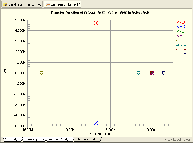
Figure 1. Accessing mixed-signal simulation analysis results, click on the relevant tab to see the results for that Analysis type.
The charts created for certain mixed-signal simulation analysis types will not contain plots and/or waveforms. For example the chart for an Operating Point analysis displays textual data. The chart for a Pole-Zero analysis contains a single plot, but graphical pole (X) and zero (0) entries rather than waveforms in the typical 'analog wave' sense.
For analyses that result in analog waveform data, the number of plots contained in a chart will depend on the analysis type and the list of signals you have added to the Active Signals list of the dialog. For example, running a Transient analysis of a circuit will display each Active Signal in its own plot, as illustrated by Figure 2. The waveform names will be as they appear in the Active Signals list.
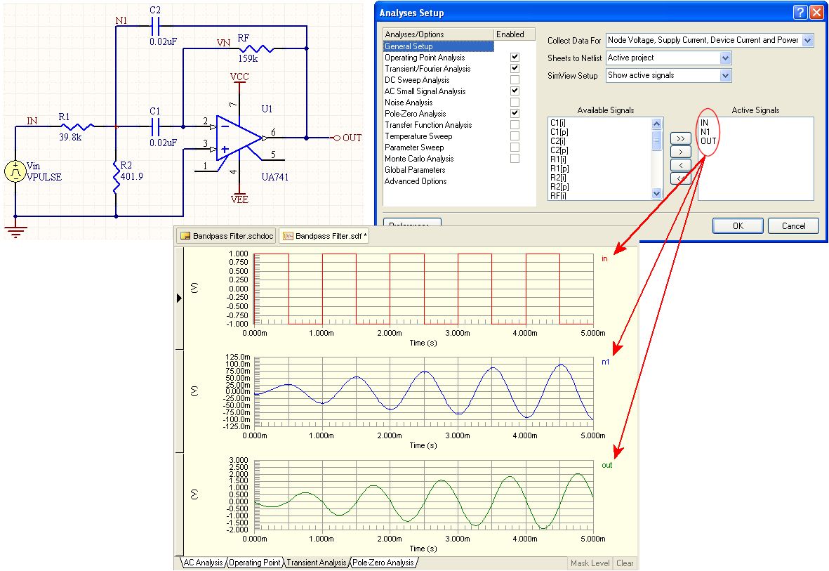
Figure 2.Each active signal is displayed in its own plot.
Displaying Multi-pass Results
Monte Carlo analysis, Parameter Sweep and Temperature Sweep are all advanced simulation features that perform multiple passes of a basic analysis type (e.g. AC Small Signal, Transient, etc), varying one or more circuit parameters with each pass. When the results are displayed within the Sim Data Editor's main analysis window, two plots will be used for each analyzed signal - one plot displaying the single waveform resulting from the use of the nominal circuit values, and one containing the multi-pass results.
For the plot containing the multi-pass results, each pass is identified by adding a letter and a number after the waveform name. The letter is used to signify the type of multi-pass analysis:
- m - Monte Carlo
- p - Parameter Sweep
- t - Temperature Sweep.
The number signifies the actual pass.
Figures 3-5 illustrate example results gained from running each of these multi-pass features.

Figure 4.Results of a Monte Carlo analysis.

Figure 5.Results of a Temperature Sweep.
For Parameter and Temperature sweep multi-pass results, as you click on the waveform name, information on the parameters(s) used in that particular pass will appear underneath the plot. For a Parameter Sweep pass, the information will be displayed in the following format:
PrimarySweepVariable = Value, SecondarySweepVariable = Value (sweep x of n).
For a Temperature Sweep pass, the information will take the form:
option[temp] = Value (sweep x of n).
In either case:
Value is the value used for a device in the circuit or the temperature set for the circuit.
x is the number of the pass selected
n is the total number of passes.
Figure 6 shows example results for a parameter sweep of a transient analysis. The currently selected waveform is out_p04, which is in fact pass 4 of an 11 pass sweep. As shown, the value for the primary sweep variable (r1resistance) on this sweep is 96.00k (Ohms).
Figure 6.Display of sweep information.
If a considerable number of passes are involved in a sweep, the analysis window will include a scroll feature. Simply click on the available button(s) to scroll through all waveform names resulting from the sweep.
Data Displayed when Performing a Signal Integrity Analysis
When performing a signal integrity analysis, a separate chart will be created for each net reflection analysis specified on the Signal Integrity panel. If a crosstalk analysis is also performed an additional, single chart, will be created.
Crosstalk analysis is only possible when performing post-layout signal integrity analysis from a PCB design document. This is because routed nets are required for this type of analysis.
The chart for a particular analysis is accessed by clicking on its named tab at the bottom of the waveform display window (Figure 7). Note that for reflection-based analysis, a chart is named after the net upon which the reflection analysis is performed.
Figure 7. Accessing signal integrity analysis results, click the Tab at the bottom to access the results for each analysis type.
Reflection Analysis Data
For a reflection analysis chart, the data displayed depends on:
- the number of pins in the net under test
- the specific termination types enabled (on the Signal Integrity panel)
- whether a sweep of the (virtual) termination component values is included as part of the analysis (again, enabled and defined on the Signal Integrity panel).
If you simply ran a reflection analysis with no termination components, a chart would contain one plot for each pin in the net under test. Each plot would contain one waveform - relating to the analysis of that pin with no termination used. For example, consider a reflection analysis for the net DTRA, which includes the following pins: - U1 pin 12
- U2 pin 4
- U2 pin 5.
With no terminations enabled, the following chart (plots and waveforms) would be created and displayed for this net.
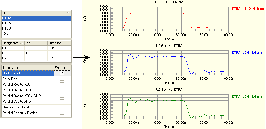
Figure 8.Reflection results - no terminations.
As you can see from Figure 8, the waveform names are created based on the net name, the specific pin and the type of termination (in the case of Figure 8, no termination).
Now, if you were to enable specific termination types, without enabling a sweep of the values, additional waveforms would be added to each plot representing the results obtained by using each of those terminations. Figure 9 shows, for emphasis, the case when all termination types are enabled.
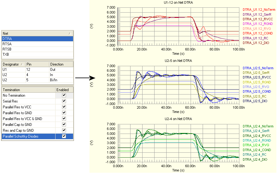
Figure 9.Reflection results - terminations enabled (no sweep).
If you enable terminations AND a sweep of the termination values (with two or more sweep steps), you will get a plot for each pin in the net under test, and for each enabled termination. The waveforms that are displayed within each plot will be those for each sweep step for that particular termination, as well as the no termination waveform (for comparison). Figure 10 illustrates this display for our example DTRA net - with two termination types enabled (Serial Res and Parallel Res to VCC), and the sweep feature enabled with Sweep Steps set to 2.
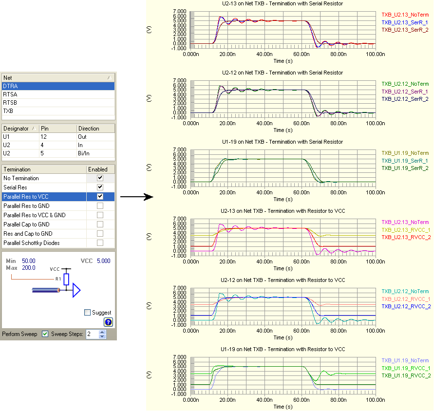
Figure 10.Reflection results - terminations enabled, with sweep.
Crosstalk Analysis Data
The display of data for the crosstalk analysis chart is essentially the same as that for a reflection analysis chart. The only difference being that as there is only a single chart for this analysis type, it will contain a plot for each pin in each net considered in the analysis. Figure 11 shows an example where two nets are considered in a crosstalk analysis - DTRA (set to be the Aggressor net) and RTSA (which defaults to being the Victim net). No specific termination types have been enabled.
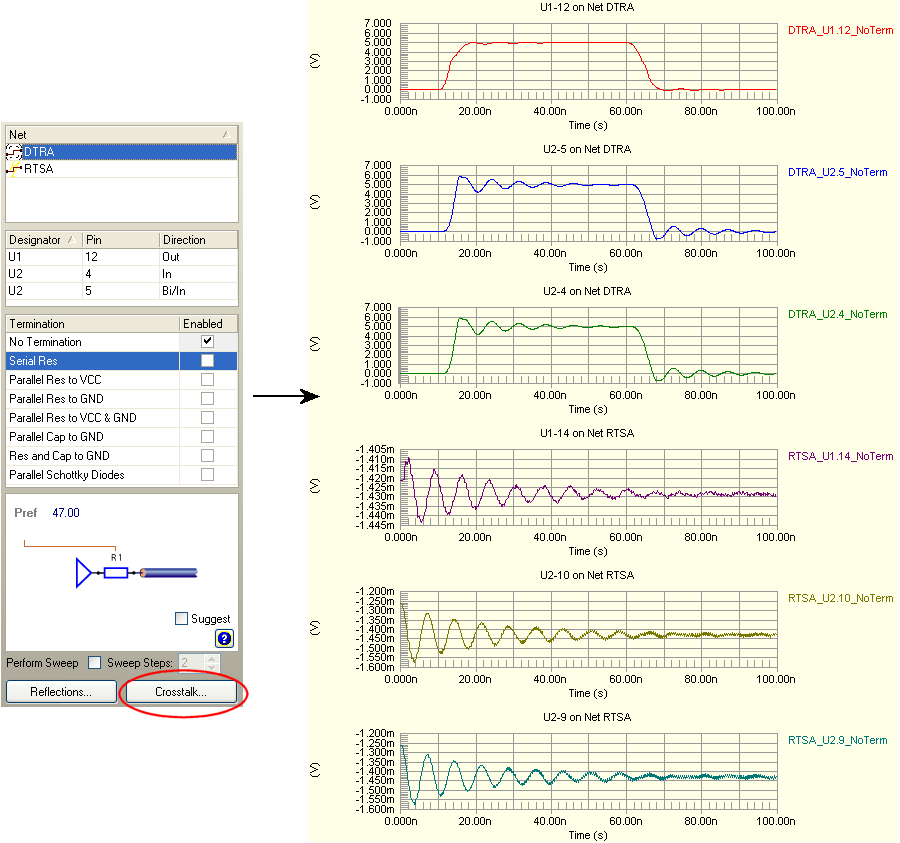
Figure 11. Crosstalk results - no terminations.
Changing the View
When analysis results are first written to an SDF file they are, by default, displayed in an optimum way - displaying between one and four plots in view at a time, depending on the number of plots resulting from the analysis. For example, if there are three plots, the chart will be configured automatically to display all three plots in view. If there were six plots, the chart would be automatically configured to display four plots in view at a time, and so on. You can change how many plots are 'visible' (i.e. displayed at any one time in the waveform analysis window) from the Document Options dialog (Figure 12). Access this dialog for the active SDF file by choosing Tools » Document Options from the main menus.
By setting the number of plots visible to All, you will typically be able to see all plots at once within the main analysis window (dependant of course on the number of plots resulting from the analysis).
Figure 13.Configuring a chart to display all plots at once.
This is considered to be a 'draft mode' - providing a quick overview of the generated waveforms. This viewing mode is especially useful if you have performed a mixed-signal simulation of a circuit whose signals are predominantly digital, allowing you to see the interaction of signals with greater ease. In fact, if at least one digital component is detected in your circuit, the display will default to this mode.
Figure 14.Comparison of digital signals is made by displaying all plots automatically.
The settings defined in the Document Options dialog can be applied to the active chart only, all charts in the current SDF file, and/or saved as the default options - which will be applied to all subsequently generated charts.
When you want to analyze the waveforms in more detail, you should move from viewing all plots, to a specific number of them. The lower the number of plots visible in the workspace at any one time, the easier it will be to concentrate on a particular waveform and take measurements from it. If you want to take advantage of resizing features (X- and/ or Y-axes), addition of Y-axes and plot labeling, you will need to set the Number of Plots Visible option (in the Document Options dialog) to anything but All.
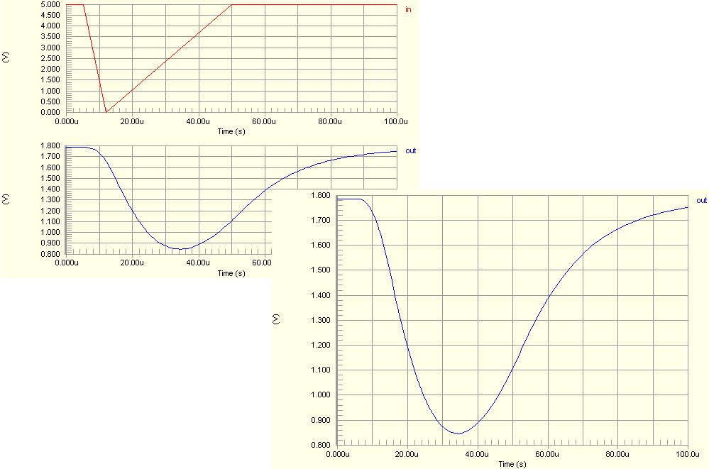
Figure 15.Setting the display to a specific number of plots.
The Document Options dialog also offers the ability to change the color scheme for a chart. This allows you to set up the workspace to meet your preferred viewing needs. Particularly useful is the Swap Foreground/Background button which, as its name suggests, allows you to quickly invert your color scheme (Figure 16).
Rearranging Plots
You can change the order in which plots appear in a chart, simply by clicking-and-dragging. This can be carried out irrespective of the view mode you are in, but is easier to do when displaying All plots.
First, ensure that the plot you wish to move is made active in the waveform analysis window. When the Number of Plots Visible is set to All (in the Document Options dialog) the active plot is distinguished by a black solid line around its waveform name section. If the Number of Plots Visible is set to 2, 3, or 4, the active plot is distinguished by a black arrow at the left hand side of its display area.
The movement of a plot is essentially the same for the different view modes:
* All plots mode - click inside the waveform name area (away from the name itself) and drag up or down as required. A black line will appear to indicate under which plot the plot you are moving will be placed, if you release the mouse button.
- Single plot mode - click anywhere to the left of the Y-axis and drag up or down as required. Again, a black line will appear to indicate the insertion point.
- 2, 3, 4 plots mode - click on the arrow at the left of the display (or anywhere to the left of the Y-axis) and drag up or down as required. Once again, a black line will appear to indicate the point of insertion.
The image below shows an example of moving a plot containing the waveform out below a plot containing the waveform in.
Figure 19.Plot rearrangement - simply click and drag.
Displaying Multiple Waveforms in a single Plot
When the analysis results are first generated, the default behavior is to display each waveform in its own plot. The exception to this would be when running sweep-based analyses. Just as plots can be moved, waveforms themselves can be moved between plots. Simply click on a waveform name and drag it to the required destination plot. A black arrow will appear at the top of the Y-axis for the recipient plot. Again, movement can be performed irrespective of the view mode (number of visible plots).
Figure 20 illustrates an example by which the waveform out is moved to share the same plot as the waveform in.
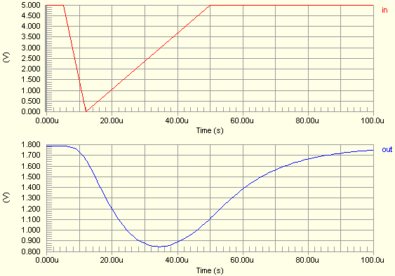
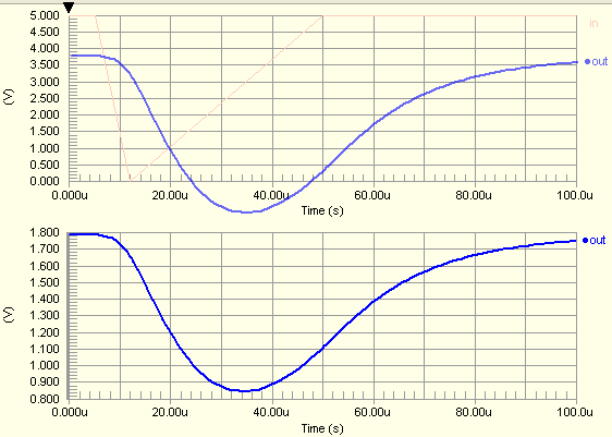
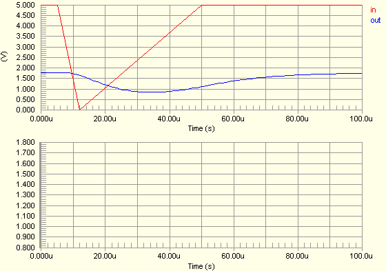
Figure 20. Drag and drop the waveforms to suit your analysis needs - here the lower blue waveform is dropped onto the upper red waveform.
You may need to adjust the Y-axis after the move, in order to better 'fit' the waveforms. This is especially true if the destination waveform is larger in amplitude than the waveform in the target plot. For more information on adjustment of plot axes, see the section Resizing Waveforms later in this document.
Magnifying the Data
You can change the magnification of the active chart, allowing you to zoom-in or out when analyzing waveform data. Use the dedicated Zoom commands to zoom-in or zoom-out respectively. Alternatively, click and drag a selection square about a point of interest to magnify (zoom-in) to that point.
As all plots in a chart have a common X-axis, changing the magnification of the data in one plot will actually cause that same level of magnification to be applied to all plots.
To zoom relative to the cursor position using the Zoom commands, position the cursor and launch the command using its keyboard shortcut - Page Up for zoom-in and Page Down for zoom-out.
To return to the initial display of the waveforms (non-magnified), simply run the View » Fit Document command from the main menus (shortcut: Ctrl+Page Down).
Adding New Charts and Plots
There may be occasions where you want to apply mathematical functions to waveforms, arrange the plots in a certain order, change the scaling of axes, or display custom-created waveforms. If you perform any of these on an existing (automatically generated) chart for an analysis, that information will be lost when you run a subsequent analysis and choose to view the results for the active signals (rather than keeping the last display setup). In such cases, you may prefer to create one or more new charts.
Create a new chart using the New Chart command, accessed from the main Chart menu. The Create New Chart dialog will appear (Figure 21). Use the dialog to define a name (which appears on its tab) and title for the chart, as well as a title and units for the X-axis. The scaling options for the X-axis will be unavailable at this time. The Cursors tab allows you to determine what data gets presented on the chart itself when using measurement cursors. These options can be defined before the chart's creation, or at a later stage by accessing the Chart Options dialog (Chart » Chart Options).
The new chart will be added, with its tab inserted to the right of the existing chart tabs.
![]()
Empty plots can also be added to a chart using the Edit » Insert command. Where plots already exist, using this command will insert a new plot above the active plot.
A newly created chart is blank by default, so you will want to populate it. The fastest way to do this would be to copy existing plots from another chart and paste them into the new chart (see next section). You can, however, create new plots from scratch.
Plot creation is performed using the Plot Wizard. Access to this wizard is made by running the command from the main Plot menu (Plot » New Plot), or by right-clicking within the chart and choosing Add Plot. Follow the pages of the wizard, including defining how the plot should appear and any waveforms that you wish to add to the plot upon its creation. After clicking Finish, the new plot will be added below the last existing plot in the chart.
Copying Charts and Plots
As mentioned, the quickest way to add a plot to a new (or existing) chart is to copy an existing one. Simply ensure that the plot you wish to copy is made active in the current chart and press Ctrl+C. It is important that a constituent waveform not be selected prior to the copy, otherwise you will simply copy the waveform instead.
When copying a plot, both the plot and its constituent waveform(s) will be included in the copy.
The plot can be pasted (Ctrl+V) into the same chart, a different chart of the same SDF file, or a chart of a completely different SDF file. When pasted, the plot will be inserted after the last plot in the chart. A copied plot can only be pasted once.
A chart itself can be copied to the Windows clipboard, for use in other applications, such as MS Word. Simply ensure that the chart you want to copy is active in the main analysis window and choose Tools » Copy to Clipboard from the main menus.
If a chart contains purely textual information, such as that for an Operating Point analysis, the information itself (rather than the whole chart display) can be copied to the clipboard, using the Tools » Copy to Clipboard as Text command.
Deleting Charts and Plots
To delete a chart, simply ensure it is the active chart in the main analysis window and either use the Chart » Delete Chart command, or right-click on the chart's tab and choose Delete Chart from the menu that appears.
To delete a plot, simply ensure it is the active plot in the current chart and either use the Plot » Delete Plot command, or right-click within the plot and choose Delete Plot from the menu that appears.
If you want to leave the plot intact, deleting only the waveforms contained therein, use the Edit » Clear command instead.
Exporting Charts and Plots
Commands available on the File » Export sub-menu allow you to export the active chart or the active plot into comma separated value (*.csv) format. In either case, the Export Data dialog will appear.
If you are exporting the active plot, all waveforms contained within that plot will be exported. You can control whether Real or Complex data is exported, and specify the delimiter to be used (comma by default).
If you are exporting the active chart, the Waves To Export region of the dialog will also be available. You have the choice of exporting only data for those waveforms currently displayed in the chart, or all waveforms for which source data is available. The latter can include signal data captured from the analyzed circuit, as well as user-defined waveforms. The Source Data region of the Sim Data panel lists all waveforms for which there is available (stored) data.
After defining export options, specify where you wish the exported file to be saved, using the Export Selected Waveforms dialog.
The exported file contains each signal waveform stored as a set of data points comprising an X-axis (time) value and a Y-axis (data) value.
For information regarding the export of individual waveforms, see the section Exporting Waveforms later in this document.
Keeping Display Setup Information
When you close the Simulation Data File, the setup information is saved with the file. If you open the file again, the arrangement of charts and plots and the waveform data within will be exactly as you left them. When running a mixed-signal circuit simulation, you have the opportunity to ensure that your SDF file setup is retained. This is done by ensuring the SimView Setup option is set to Keep last setup, in the Analyses Setup dialog.
If, when you re-run a simulation, you want it to display the analyses and nodes that you have just setup - in the Analyses Setup dialog - change the SimView Setup option to Show active signals.
Waveform Management
The previous pages of this document have looked at how the results of an analysis are displayed within the analysis window and how features of the Sim Data Editor allow you to change and setup the display to meet your requirements. We also touched on the ability to move waveforms between plots as part of changing the display. This section of the document delves deeper into the waveforms themselves and, more importantly, the host of features provided by the Editor to manage them.
Selecting a Waveform
Selection of a waveform within the main analysis window is simply a case of clicking on the waveform's name. Once selected, the waveform will become bolder in color and have a dot to the left of its name. Filtering is applied, using the name of the waveform as the scope. All other waveforms in the active chart with different names will be masked (becoming dimmed).
If more than one waveform of the same name exists in the active chart, the non-selected instances will remain at full visibility.
Figure 25. Selection of a waveform.
The extent of the masking can be controlled through use of the Mask Level slider bar, accessed by clicking the Mask Level button, located at the bottom-right of the analysis window.
Formatting a Waveform
Format a selected waveform using the Format Wave dialog - accessed either by choosing Wave » Wave Options from the main menus, or by directly right-clicking on the waveform's name and choosing Format Wave from the pop-up menu that appears.
The dialog allows you to:
- Change the name for the waveform. This is the name as it appears in the main analysis window. The actual name for the captured source data signal is not changed.
- Change the units used for the waveform's Y-axis.
- Change the color used for the waveform. This can be especially useful when a plot contains multiple waveforms and you want to make the plot as 'readable' as possible.
Resizing Waveforms
The waveforms are automatically scaled when they are first displayed. The Y-axis of each plot is scaled such that all waveforms in the chart are fully visible.
When running a signal integrity analysis, the extent of the X-axis is determined by the Total Time (s) option, set on the Configuration tab of the Signal Integrity Preferences dialog (accessed from the Signal Integrity panel).
The X-axis will be scaled in accordance with the setting for the particular analysis type. For example the extent of the X-axis when running a Transient analysis is defined by Transient Stop Time - Transient Start Time. For an AC Small Signal analysis, the extent would be Stop Frequency - Start Frequency.
Changing the X-axis
The X-axis is common to all plots in a chart. You cannot change the scaling of the X-axis for an individual plot. Scaling for the X-axis is changed from the Scale tab of the Chart Options dialog. Fast access to this tab can be made by double-clicking on the X-axis of any plot in the active chart.
In the X Axis Scale region of the dialog, uncheck the checkboxes if you want to apply your own, manual scaling. Use the Minimum and Maximum fields to change the extents of the X-axis. Change the Division Size to expand or contract the waveforms horizontally.
For waveforms obtained by running an AC Small Signal analysis, make use of the Grid Type options in the dialog to change the X-axis from Linear to Logarithmic (base 2 or base 10).
Changing the Y-axis
Changing the scaling of the Y-axis for one plot will not affect the scaling of the Y-axis for another. Simply put, the Y-axis is local to each plot in a chart. Scaling for the Y-axis is changed from the Y Axis Settings dialog. Fast access to this dialog can be made by double-clicking on the Y-axis for a plot.
In the Scale region of the dialog, uncheck the checkboxes if you want to apply your own, manual scaling. Use the Minimum and Maximum fields to change the extents of the Y-axis. Change the Division Size to expand or contract the waveforms vertically.
The Y Axis region of the dialog allows you to add a label to the axis. By default, the units used for the axis come directly from the Units field in the Format Wave dialog. If more than one waveform share a plot, the units will only be shown (when the waveforms are not selected) if the units for each waveform are the same. Otherwise units will only be shown as each waveform is selected. Disable the Auto option and manually enter units as required.
To quickly display all waveforms in their entirety, use the View » Fit Document command (Shortcut: Ctrl + Page Down).
The Y-axes cannot be changed when the chart is configured to display All plots.
Defining Multiple Y-axes for a Plot
There may be times where a single Y-axis will just not work. For example, you may be wanting to contrast current and voltage signals in a common plot. The voltage signal might run to 5V, whereas the current signal may be in the order of milliamps or microamps. To make the waveforms 'readable' the Sim Data Editor provides for the use of additional Y-axes. Consider the waveforms shown in the image above. One shows the voltage across a resistor (R1) and the other shows the current through that resistor.
If the current waveform is now moved into the same plot as the voltage waveform (shown above), you can see that the current waveform is basically lost when scaled using the existing Y-axis for the plot. A better approach is to define a new Y-axis, giving the result shown below.
A new Y-axis can be added for the current waveform in one of the following ways:
- right-click on its name, choose Edit Wave, and in the Edit Waveform dialog that appears enable the Add to New Y axis option.
- add a new Y-axis (Plot » Add Y Axis), then drag the current waveform onto the axis to create association.
The new (automatically scaled) Y-axis for the waveform will be added to the left of the existing Y-axis. The result (Figure 31) is easily readable waveforms in a single plot.
Removing a Y-axis
To remove a Y-axis from a plot that has multiple Y-axes defined for it, simply click on the axis to select it and run the Plot » Remove Y Axis command. Alternatively, right-click on the axis and choose Delete Axis from the menu that appears.
Displaying a Waveform Scaled Two Ways
When running an AC Small Signal analysis, you will often need to analyze and simultaneously display the same waveform scaled in different ways. For example you may need to display the output both in terms of frequency and phase.
Consider the waveforms in the image on the left below, acquired by running an AC analysis on a Bandpass Filter circuit.

It is the output waveform that we are most interested in and we would like to simultaneously compare the frequency (in Decibels) with the phase (in Degrees). We can easily display these two variants of the output waveform in separate plots. We can quickly lay the foundation for this by removing the input waveform and replacing it with a copy of the output waveform (image above on the right).
One waveform needs to be changed to show the output frequency of the circuit in DBs instead of Hz. The other needs to show the phase of the output. Both are achieved using the Complex Functions available in the Edit Waveform dialog (right-click on a waveform name and choose Edit Wave).
For the top waveform, enable Magnitude (dB). For the bottom waveform, enable Phase (Deg). The resulting waveforms are shown in the image below.
Figure 35. Displaying magnitude and phase of the output waveform.
For ease of analysis, the waveforms could also be overlayed in the same plot, with a separate Y-axis used for each (Figure 36).
Figure 36. Magnitude and phase displayed within same plot using separate Y-axes.
Editing Waveforms - Getting Mathematical
As part of the analysis of your design you may want to perform a mathematical operation on one or more of the analysis signals, and view the resultant waveform. You can in fact construct a mathematical expression based on any of the source data waveforms.
To edit a waveform in this way, simply right-click on its name and choose Edit Wave (or select the waveform and choose Wave » Edit Wave from the main menus). The Edit Waveform dialog will appear.
The dialog provides:
- a list of currently available waveforms
- a list of available functions
- an expression building field.
An expression can be constructed by typing directly into the Expression field, or by clicking to select a function in the Functions list, then clicking to select the signal that you want to apply that function to.
The expression can include any combination of available functions and allowed operators, and be assigned a meaningful name with which the resultant waveform will be referenced in the plot. - The best way to demonstrate the use of mathematical expressions is by example. Consider the sinusoidal waveform (in) in Figure 38.
Figure 38. Base sinusoidal waveform (unedited).
A simple expression to test the use of functions might be:
COS ^2^ (in) + SIN ^2^ (in) = 1 to which we would expect the resultant waveform to be a horizontal line at the value of 1V.
Figure 39 shows both the entry for the expression in the Edit Waveform dialog, and the resulting waveform - which is as expected!
Figure 39. Waveform after application of mathematical expression.
The functions available will depend on the analysis type run to obtain the waveforms. For analyses like AC Small Signal, the dialog will provide a range of complex functions, allowing you to quickly change the waveform to show magnitude in DBs, or phase, or even group delay. The following sections detail each of these general and complex functions.
For an example of using complex functions with the results of an AC analysis, see the previous section Displaying a Waveform Scaled Two Ways.
Available Functions - General
The following general functions and operators are provided in the Edit Waveform dialog. The actual functions available will depend on the analysis type.
| ( ) | Precedence indicators. Use to set precedence of math operations. Operations contained within ( ) will be performed first. |
| + | Addition operator. |
| - | Subtraction operator. |
| * | Multiplication operator. |
| / | Division operator. |
| ^ | Power operator, y^x returns the value of "y raised to the power of x". This function is the same as PWR( , ). |
| ABS( ) | Absolute value function. ABS returns the value of |x|. |
| ACOS( ) | Arc cosine function. |
| ACOSH( ) | Hyperbolic arc cosine function. |
| ASIN( ) | Arc sine function. |
| ASINH( ) | Hyperbolic arc sine function. |
| ATAN( ) | Arc tangent function. |
| ATANH( ) | Hyperbolic arc tangent function. |
| AVG( ) | Average function. Returns the running average of the wave data. |
| BOOL( , ) | Boolean function. In the expression BOOL(wave, thresh), wave would be the name of a waveform, thresh would be the switching threshold. Returns a value of 1 for wave arguments greater than or equal to thresh and 0 for wave arguments less than thresh. |
| COS( ) | Cosine function. |
| COSH( ) | Hyperbolic cosine function. |
| DER( ) | Derivative function (dx/dt). Returns the slope between data points. |
| EXP( ) | Exponential function. EXP returns the value of "e raised to the power of x", where e is the base of the natural logarithms. |
| INT( ) | Integral function. Returns the running total of the area under the curve. |
| LN( ) | Natural logarithm function, where LN(e) = 1. |
| LOG10( ) | Log base 10 function. |
| LOG2( ) | Log base 2 function. |
| PWR( , ) | Power function. Same as |
| RMS( ) | Root-Mean-Square function. Returns the running AC RMS value of the wave data. |
| SIN( ) | Sine function. |
| SINH( ) | Hyperbolic sine function. |
| SQRT( ) | Square root function. |
| TAN( ) | Tangent function. |
| TANH( ) | Hyperbolic tangent function. |
| UNARY( ) | Unary minus function. UNARY returns -x. |
| URAMP( ) | Unit ramp function. Integral of the unit step: for an input x, the value is zero if x is less than zero, or if x is greater than zero, the value is x. |
| USTEP( ) | Unit step function. Returns a value of one for arguments greater than zero and a value of zero for arguments less than zero. |
Available Functions - Complex
The following complex functions are provided in the Edit Waveform dialog. Again, availability of these functions depends on the particular analysis type (e.g. AC Small Signal analysis).
| Magnitude | Returns the magnitude of the wave. |
|---|---|
| Magnitude (dB) | Returns the magnitude of the wave expressed in Decibels. |
| Real | Returns the real component of a complex waveform. |
| Imaginary | Returns the imaginary component of a complex waveform. |
| Phase (Deg) | Returns the phase of the wave expressed in degrees. |
| Phase (Rad) | Returns the phase of the wave expressed in radians. |
| Group Delay | Returns the group delay for the wave. |
Fast Fourier Transform
By using the Chart » Create FFT Chart command, you can quickly perform a Fast Fourier Transform on each waveform in the active chart. The results are stored in, and displayed on, a new chart, which is named using the format SourceChartName_FFT and added to the right of the existing charts in the SDF file.
Set the FFT Length in the Document Options dialog (Tools » Document Options). By default the length is 128.
Creating a New Signal Waveform
As well as source data waveforms generated as a result of running an analysis on a circuit (simulation) or design (signal integrity), you also have the opportunity to create your own waveforms. Access to the waveform creation feature is made through the Source Data dialog. Access this dialog from the main menus (Chart » Source Data) or by clicking the Source Data button on the Sim Data panel.
Once you have the Source Data dialog open, simply click the Create button. The Create Source Waveform dialog will appear (Figure 41). From this dialog you can create:
- A sinusoidal-based waveform
- A pulse-based waveform
- A user-defined waveform based on entry of a set of data points, with each point defined using an XY value pair.
Once you have finished defining the new waveform as required, give it a meaningful name and click OK - it will be added to the list of source data waveforms.
User-defined waveforms (i.e. those not generated through circuit analysis) can be edited at any stage, with respect to their characteristics. Simply select the waveform's entry in the list and click the Edit button.
Storing and Recalling Waveforms
The Sim Data Editor provides the ability to store and recall waveform source data. Access to the storage feature can be made in two ways:
- Directly from the main analysis window. Simply select the waveform you wish to store and choose Tools » Store Waveform from the main menus.
- From the Source Data dialog (Chart » Source Data). Simply select the waveform you wish to store from the list and click the Store button.
The waveform will be stored in an ASCII file (*.wdf) as a set of data points, with each point being represented by an XY value pair. Use the subsequent Store Selected Waveform dialog to nominate where, and under what name, you want the file saved. By default, the file will be named using the actual name of the waveform (i.e. WaveformName.wdf).
Recalling a waveform that has been previously stored can also be performed in two ways: - Directly from the main analysis window. Choose Tools » Recall Waveform from the main menus.
-
From the Source Data dialog - click the Recall button.
Tip:If a waveform is recalled that possesses the same name as an existing waveform in the source data list, it will be given the suffix _1. Subsequent recall of the same waveform will result in waveforms appearing in the list with incremented suffixes (_2, _3, etc).
Use the subsequent Recall Stored Waveform dialog to browse to and open the required WDF file. The waveform will be recalled and loaded into the source data list for the active chart.
Copying Waveforms
A waveform can be readily copied and pasted using the standard Ctrl+C and Ctrl+V shortcuts respectively. Ensure that the waveform is selected before copying.
The waveform can be pasted into a plot of the same chart, a plot of a different chart in the same SDF file, or a plot in a chart of a completely different SDF file. When pasting, ensure that the target plot is currently the active plot in the chart. The recipient plot can be empty or it can contain one or more existing waveforms. A copied waveform can only be pasted once.
After pasting a copied waveform, you can move it to a different plot as required. If you want to move the waveform to its own plot and there is no empty plot existing in the chart, change the view mode to show All plots visible (from the Document Options dialog), then simply drag the waveform to a point beyond the last plot in the chart - a new plot will automatically be added.
If pasting between charts, the pasted waveform may, at first sight, look incorrect. This may be due to the time base (X-axis) being different between source and destination charts.
Deleting Waveforms
To delete a waveform from a plot, simply ensure it is selected and either use the Wave » Remove Wave command, or right-click on the waveform's name and choose Remove Wave from the menu that appears. Alternatively, select the waveform and hit the Delete key.
Deleting Waveforms Permanently
Deleting a waveform using one of the techniques listed in the previous section simply removes that waveform from the waveform analysis window. The captured data for the waveform is not deleted. The waveform remains listed as part of the available source data for the active chart. Permanent removal of waveforms is carried out from the Source Data dialog. Access this dialog from the main menus (Chart » Source Data) or by clicking the Source Data button in the panel.
To permanently delete a waveform, simply select its name in the list and click on the Delete button. Multiple waveforms may be selected for deletion using the standard Ctrl+click, Shift+click and click-and-drag features.
To bring back a waveform that has been deleted in this fashion, you would either need to recall a stored copy of it (from a *.wdf file), or re-run the analysis.
Exporting Waveforms
A selected waveform may be exported into comma separated value (*.csv) format by using the File » Export » Waveform command. Use the Export Data dialog that appears to define export options as required, then use the subsequent Export Selected Waveforms dialog to specify where the exported file is to be saved.
The exported file contains the signal waveform stored as a set of data points comprising an X-axis (time) value and a Y-axis (data) value.
Importing Waveforms
Waveform data stored in comma separated value format (*.csv) can be easily imported into the active chart. This allows you to quickly import data that has been previously exported, or to import waveform data that has been generated from a third party application - as long as it has been stored in CSV format.
Before importing, first ensure that the chart you wish to import into is made active in the main analysis window. Access the import feature by running the File » Import command. Use the subsequent dialog that appears to browse to and open, the required CSV file. The remaining steps of the import are all carried out using the Import Data Wizard (Figure 45). Follow the pages of the wizard - upon clicking Finish the waveforms will be imported into the active chart and be added to that chart's source data list.
If any of the waveforms being imported have names matching those already existent for the recipient chart, the wizard will alert you to this fact, listing the offending waveforms, and asking for you to rename the imported version of those signals. Click directly on a name in the wizard to edit it.
Displaying Data Points
If you are unsure about the accuracy of the waveforms - perhaps they look sharp and jagged instead of smooth and curved - you can enable the display of data points, to check if the results have been calculated often enough.
To display these points, simply enable the Show Data Points option in the Document Options dialog. A small circle will be displayed at each point along the wave at which data was calculated (Figure 46).
Identifying Waveforms on a Monocolor Print
With the ability to assign any color you want to a waveform, display of multiple waveforms within the same plot is kept manageable when viewing results and distinguishing between waveforms in the Sim Data Editor. However if the results are printed in monochrome, color assignment, on the whole, becomes redundant.
To make each waveform on a single color printout easily identifiable, the Viewer provides a feature to add identifier symbols to each waveform. To display these symbols, simply enable the Show Designation Symbols option in the Document Options dialog. If the waveforms are displayed in individual plots, then a square symbol will be used for each. If two or more waveforms are displayed within the same plot, then a different shape is used for each (Figure 47).
Cross Probing
The Sim Data Editor offers the ability to cross-probe from the selected waveform to the corresponding analysis node in the circuit from which the results for that waveform were captured. Cross probing will either be to a schematic or a PCB, depending on where the analysis was performed.
Cross Probing to the Schematic
You can only cross probe from waveforms for which data was captured through analysis of the schematic circuit. If you have edited a source waveform by applying a mathematical expression to it, or if you have created a new waveform, you will not be able to cross probe.
To use this feature, simply right-click on the name of a waveform in the main analysis window and choose Cross Probe to Schematic from the pop-up menu that appears. The source schematic document will be made active and the corresponding node highlighted - in accordance with the Highlight Methods defined on the System - Navigation page of the Preferences dialog.
Figure 48 illustrates an example of cross probing to a schematic, where the portion of the circuit associated with the OUT net is highlighted.
Cross Probing to the PCB
The ability to cross probe from a selected waveform to a PCB is available if you have performed a post-layout signal integrity analysis of your design.
To cross probe, simply right-click on the required waveform name and choose the Cross Probe to DocumentName.PcbDoc command. The PCB document will be made active and the corresponding pin for the analyzed net will be highlighted, again in accordance with the Highlight Methods defined on the System - Navigation page of the Preferences dialog.
the image above illustrates an example of cross probing to a PCB, where pin 10 of component U2 - associated with net RTSA - is highlighted.
Taking Direct Measurements
The Sim Data Editor provides features for obtaining measurement information directly within the main analysis window. Base measurements are automatically presented for a selected waveform. If you want to take more precise measurements, dedicated measurement cursors are available - enabling you to take measurements in a more interactive way.
Measurements for a Selected Waveform
General measurements for a selected waveform are presented in the Waveform Measurements region of the Sim Data panel.
Figure 50. General measurements for a selected waveform.
Data is calculated from the waveform itself and does not involve the measurement cursors in any way. The following data is calculated:
| Rise Time | The time taken to rise to the steady state value for the high level of the signal waveform (top line). Measurement data is only available when the selected signal is power-based (mixed-signal simulation) or is a resultant waveform of a signal integrity analysis. |
| Fall Time | The time taken to fall to the steady state value for the low level of the signal waveform (base line). Measurement data is only available when the selected signal is power-based (mixed-signal simulation) or is a resultant waveform of a signal integrity analysis. |
| Min | The minimum value reached by the waveform. The X-axis value at which this point occurs is also displayed. |
| Max | The maximum value reached by the waveform. The X-axis value at which this point occurs is also displayed. |
| Base Line | The steady state value for the low level of the signal waveform. This value is most noticeable, graphically, for a signal integrity-based analysis waveform, where ringing of the signal occurs about this base line value (undershoot). |
| Top Line | The steady state value for the high level of the signal waveform. This value is most noticeable, graphically, for a signal integrity-based analysis waveform, where ringing of the signal occurs about this top line value (overshoot). |
Cursor-based Measurements
Precise data measurements can be taken by using the Sim Data Editor's dedicated measurement cursors. Two cursors are available - Cursor A and Cursor B - which can be added to the same or different waveforms in the main analysis window.
A cursor (A or B) can only be used once in the active chart. If you choose to assign a cursor to a waveform and another waveform is already using that cursor, the cursor will be reassigned to the new one.
Addition of a measurement cursor can be made in one of two ways:
- Select the waveform and use the Wave » Cursor A or Wave » Cursor B command.
- Right-click on the waveform's name and choose Cursor A or Cursor B from the menu that appears.
An added cursor will appear as a tab at the top of the plot in which the waveform resides, and will assume the same color as the waveform to which it is assigned. Crosshairs appear within the plot, intersecting the waveform. Move the cursor by clicking and dragging its tab.
Measurement data is available in the Measurement Cursors region of the Sim Data panel. You can also enable display of measurement data within the main analysis window. This is done from the Cursors tab of the Chart Options dialog (Chart » Chart Options).
The availability of cursor measurements - both in the main analysis window and on the Sim Data panel - depends on how the measurement cursors have been assigned. If a single cursor is being used, you can read just the XY values of the cursors' intersect point.
If the two cursors have been added, to different waveforms, you can measure:
- XY values
- B-A.
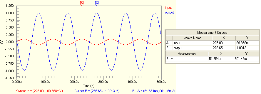
Figure 52.Using two measurement cursors - different waveforms.
If the two cursors have been added, to the same waveform, you can measure:
As you move the mouse pointer over the area of a plot, the XY value pair is shown at the far left of Altium Designer's Status bar.
- XY values
- B-A
- Minimum A..B
- Maximum A..B
- Average A..B
- AC RMS A..B
- RMS A..B
- Frequency A..B
Figure 53. Using two measurement cursors - same waveform.
Printing Analysis Results
Printing your analysis results is simply a case of following these steps:
- Ensure the chart from which you wish to print results is active in the main analysis window.
- Setup the page properties
- Setup the printer
- Preview the print (optional)
- Print
Although there are various commands available from the main File menu for these steps, you can access all required setup dialogs from the SimView Print Properties dialog (File » Page Setup).
Use this main dialog to set paper size, scaling and the output color for the print. If you are printing in Mono or Gray and have plots involving multiple waveforms, designation symbols will automatically be added to the plot.
Click the Printer Setup button to access the Printer Configuration for dialog, a standard dialog for choosing the device you want to print to and setting related properties accordingly.
Click the Advanced button in the SimView Print Properties dialog to access the Wave Print Properties dialog. Use this dialog to choose which plots in the chart are to be printed, which waveforms within those plots should be printed, and how page numbering should appear.
You can also specify which measurement data to be included in the printout. Print cursor based measurement data will only be available if you have enabled cursors in your chart. The actual measurement types depend on how the cursors have been assigned (see the Cursor-based Measurements section).
Clicking the Preview button will load the data to be printed into the Previewer dialog. Use this dialog to browse through the information you have requested to print.
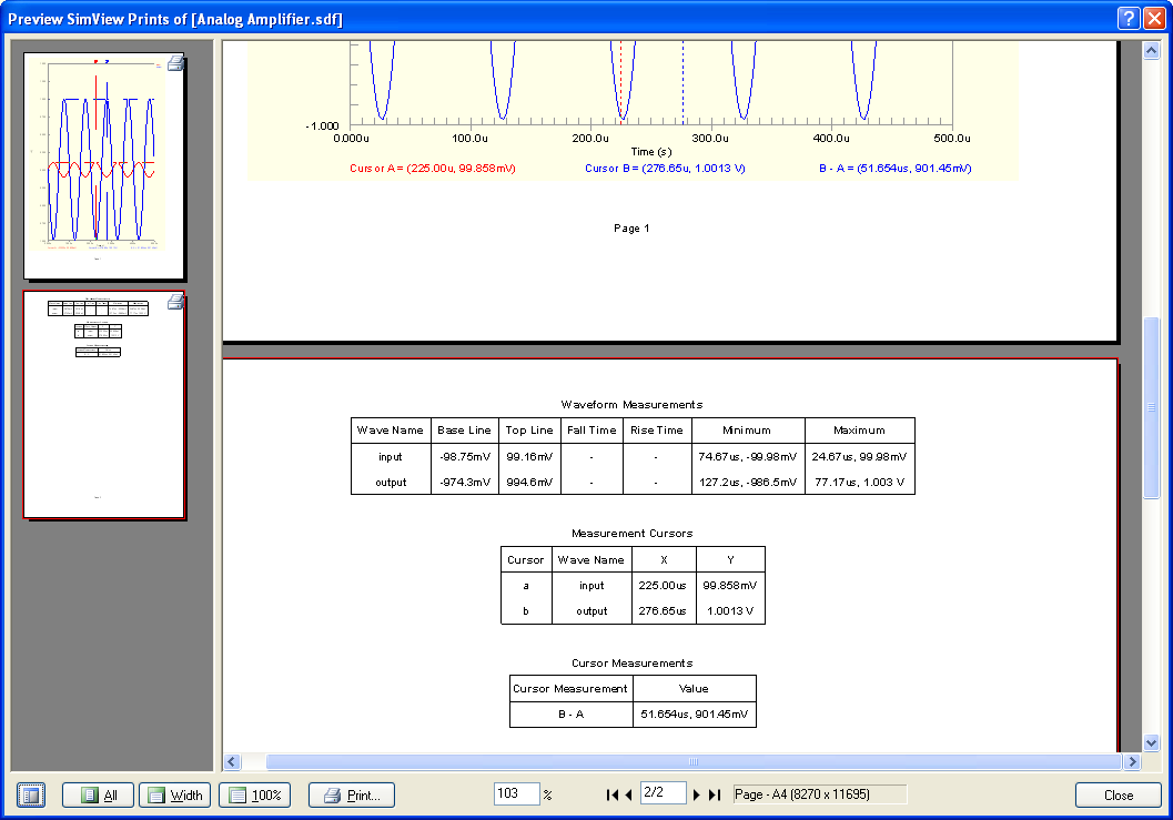
When you are satisfied that the prints are as required, simply run the Print command - either from the Previewer dialog, the File menu, or the SimView Print Properties dialog.